
A collection of R features that are typically discussed in neither R courses nor contemporary books about R.
In addition to row names and column names each element of a matrix can have its own name too. R doesn’t seem to want that to happen, and so, when a vector is turned into a matrix all the names are removed.
vec <- 1:9
names(vec) <- paste0("e", 1:9)

## e1 e2 e3 e4 e5 e6 e7 e8 e9
##  1  2  3  4  5  6  7  8  9


mat <- matrix(vec, ncol=3)

##
##      [,1] [,2] [,3]
## [1,]    1    4    7
## [2,]    2    5    8
## [3,]    3    6    9
However, they can be added manually afterwards.
names(mat) <- paste0("e", 1:9)

##      [,1] [,2] [,3]
## [1,]    1    4    7
## [2,]    2    5    8
## [3,]    3    6    9
## attr(,"names")
## [1] "e1" "e2" "e3" "e4" "e5" "e6" "e7" "e8" "e9"
And those names can be used to select the elements.
mat["e3"]

## e3
##  3


mat[c("e2","e4")]

## e2 e4
##  2  4
Sadly, they are dropped after subsetting, which makes it hard to exploit this feature for any practical use.
mat[1:2,]

##      [,1] [,2] [,3]
## [1,]    1    4    7
## [2,]    2    5    8
Indices from a matrix can be obtained in a <row, column> table form.
This format, instead of returning a single index for each match in a matrix, returns the positions by their row and column coordinates.
mat <- matrix(11:16, nrow=2)

##      [,1] [,2] [,3]
## [1,]   11   13   15
## [2,]   12   14   16


which(mat > 13)

## [1] 4 5 6


which(mat > 13, arr.ind=TRUE)

##      row col
## [1,]   2   2
## [2,]   1   3
## [3,]   2   3
And this special format can also be used to select elements from a matrix.
inds <- rbind(c(1,2), c(2,1))
mat[inds]

## [1] 13 12
Matrix can contain various classes. Below is an example - matrix of data frames.
mat <- matrix(list(iris, mtcars, USArrests, chickwts), ncol=2)

##      [,1]    [,2]
## [1,] List,5  List,4
## [2,] List,11 List,2
To select the data frame from second row, second column:
mat[[2,2]]

##   weight      feed
## 1    179 horsebean
## 2    160 horsebean
## 3    136 horsebean
## ...  ...       ...
Taking sums and means of rows or columns of a matrix is an often repeated operation.
mat <- matrix(rnorm(200), nrow=10, ncol=20)

colMeans(mat)
rowMeans(mat)
colSums(mat)
rowSums(mat)
But R also has handy functions for repeating these operations on a flattened matrix, given that the dimensions are known.
vec <- as.numeric(mat)

.colMeans(vec, m=10, n=20)
.rowMeans(vec, m=10, n=20)
.colSums(vec, m=10, n=20)
.rowSums(vec, m=10, n=20)
split() and unsplit() is a somewhat convenient way to do split-apply-combine tasks in base R.
During this procedure the data frame is first split into a list of data frames - one for each group.
Then a function is applied to all the data frames in a list.
And finally the list is recombined again to a single data frame.
dfs <- split(iris, iris$Species)
dfs <- lapply(dfs, transform, Sepal.Length=as.vector(scale(Sepal.Length)))
dfs <- unsplit(dfs, iris$Species)

##   Sepal.Length Sepal.Width Petal.Length Petal.Width Species
## 1   0.26667447         3.5          1.4         0.2  setosa
## 2  -0.30071802         3.0          1.4         0.2  setosa
## 3  -0.86811050         3.2          1.3         0.2  setosa
## 4  -1.15180675         3.1          1.5         0.2  setosa
## 5  -0.01702177         3.6          1.4         0.2  setosa
## 6   1.11776320         3.9          1.7         0.4  setosa
## ...........................................................
However it is possible to do all of this with a single call to a split()<- function:
df <- iris
split(df$Sepal.Length, df$Species) <- tapply(df$Sepal.Length, df$Species, scale)

##   Sepal.Length Sepal.Width Petal.Length Petal.Width Species
## 1   0.26667447         3.5          1.4         0.2  setosa
## 2  -0.30071802         3.0          1.4         0.2  setosa
## 3  -0.86811050         3.2          1.3         0.2  setosa
## 4  -1.15180675         3.1          1.5         0.2  setosa
## 5  -0.01702177         3.6          1.4         0.2  setosa
## 6   1.11776320         3.9          1.7         0.4  setosa
## ...........................................................
Or for all the columns in one go:
df <- iris
split(df[,1:4], df$Species) <- Map(scale, split(df[,1:4], df$Species))

##   Sepal.Length Sepal.Width Petal.Length Petal.Width Species
## 1   0.26667447   0.1899414   -0.3570112  -0.4364923  setosa
## 2  -0.30071802  -1.1290958   -0.3570112  -0.4364923  setosa
## 3  -0.86811050  -0.6014810   -0.9328358  -0.4364923  setosa
## 4  -1.15180675  -0.8652884    0.2188133  -0.4364923  setosa
## 5  -0.01702177   0.4537488   -0.3570112  -0.4364923  setosa
## 6   1.11776320   1.2451711    1.3704625   1.4613004  setosa
## ...........................................................
Possibility to create a custom infix operators by using the %...% syntax is well known.
Here is an example of the operators opposite of %in%.
`%out%` <- function(x, y) !(x %in% y)

LETTERS[LETTERS %out% c("A", "E", "I", "O", "U")]
It is also possible to create a custom assigning function, similar to names(x)<-.
As an example here is a function that can replace the first element of a vector.
`first<-` <- function(x, value) c(value, x[-1])

x <- 1:10
first(x) <- 0
However, a more surprising construct is a combination of the two. Here is an example of a function that can replace all elements falling outside of specified set(1).
`%out%<-` <- function(x, y, value) {x[!(x %in% y)] <- value; x}

x <- 1:10
x %out% c(4,5,6,7) <- 0
Maybe even more surprising is that this can be used on standard operators (those without %...%).
Below is a function that modifies the first argument of a product so that the product is equal to the given value.
`*<-` <- function(x, y, value) x*value/(x*y)

x <- 5
y <- 2

x * y
## 10

x * y <- 1

x * y
## 1
And here is an even bigger contraption - assignment from both sides:
`<-<-` <- function(x, y, value) x <- paste0(y, "_", value)

"start" -> x <- "end"

x
## "start_end"
A somewhat hidden feature of lm() is that it accepts Y in a matrix format and does regression for each column separately.
Doing it this way is also a lot faster compared to executing lm() on each column individually.
Below is an example of regressing each variable in iris dataset against Species.
This results in estimating the coefficients of 4 separate linear models.
lm(data.matrix(iris[,-5]) ~ iris$Species)

## Call:
## lm(formula = data.matrix(iris[, -5]) ~ iris$Species)
##
## Coefficients:
##                         Sepal.Length  Sepal.Width  Petal.Length  Petal.Width
## (Intercept)             -8.346e-17     2.555e-16    3.243e-16     2.853e-16
## iris$Speciesversicolor   1.316e-16    -5.809e-16    1.191e-16    -7.439e-16
## iris$Speciesvirginica   -4.441e-17    -7.772e-16    1.998e-16     3.775e-16
R has over 650 named colors.
colors()
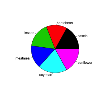
palette() allows to change the colors represented by numbers.
palette(c("cornflowerblue", "orange", "limegreen", "pink", "purple", "grey"))
pie(table(chickwts$feed), col=1:6)
And to restore the colors:
palette("default")
pie(table(chickwts$feed), col=1:6)
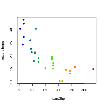
Sometimes it is necessary to color a numeric variable by its value.
For this purpose colorRamp can create a function that will interpolate a given set of colors to the [0,1] interval.
Then we can obtain a color corresponding to any number between 0 and 1.
pal <- colorRamp(c("blue", "green", "orange", "red"))

rgb(pal(0.5), max=255)
And here it is used to color the points by horse power:
# first - transform hp to a range 0-1
hp01 <- (mtcars$hp - min(mtcars$hp)) / diff(range(mtcars$hp))

plot(mtcars$hp, mtcars$mpg, pch=19, col=rgb(pal(hp01), max=255))
Sometimes it is convenient to place a plot within a plot.
One way to achieve this is with split.screen():
figs <- rbind(c(0.0, 1.0, 0.0, 1.0),
              c(0.3, 0.5, 0.6, 0.8)
              )
screenIDs <- split.screen(figs)

screen(screenIDs[1])
barplot(1:10, col="lightslategrey")

screen(screenIDs[2])
par(mar=c(0,0,0,0))
pie(1:5)

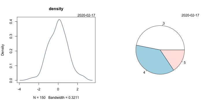
Hooks are a mechanism for injecting a function after a certain action takes place.
They are sparsely used within R.
For the demonstration plot.new hook(2) will be used here.
This hook allows user to insert an action at the end of the plot.new() function.
Here it will be used for adding a date stamp to every created plot.
setHook("plot.new", function() {mtext(Sys.Date(), 3, adj=1, xpd=TRUE)}, "append")
Now all plots should have a date:
par(mfrow=c(1,2))

plot(density(iris$Sepal.Width), lwd=2, col="lightslategrey", main="density")
pie(table(mtcars$gear))
Dollar operator $ is used to select elements from a list by name.
However it is a generic method and can be modified.
Here is a rewriting of $ operator to select rows, instead of columns, from data.frames:
`$.data.frame` <- function(x, name) {x[rownames(x)==name,]}

USArrests$Utah
##      Murder Assault UrbanPop Rape
## Utah    3.2     120       80 22.9
Auto-completion after pressing tab can also be added by rewriting the .DollarNames method:
.DollarNames.data.frame <- function(x, pattern="") {
  grep(pattern, rownames(x), value=TRUE)
}


> USArrests$A <tab>
...labama   ...laska    ...rizona   ...rkansas
To add more weirdness tab autocompletion can be made to auto-correct row name mistakes:
.DollarNames.data.frame <- function(x, pattern="") {
  agrep(pattern, rownames(x), value=TRUE, max.distance=0.25)
}

> USArrests$Kali <tab>
> USArrests$California