
Real world data analysis projects are often complicated. They can involve multi-gigabyte input files, complex data cleaning procedures, week-long computations, and elaborate reports. Hence, data science practitioners need to be able to make changes without restarting the whole pipeline from scratch. Workflow management becomes essential and many projects turn to build automation tools like Make(1). In this article I describe my approach for dealing with this problem, which is based on a lesser known build automation tool - redo(2).
Redo is a build automation system that promises to be simpler and more powerful than Make. Unlike Make or its derivatives redo is tiny, recursive, and has no special syntax of its own. It allows declaring dependencies straight from within the file that is being executed, which enables writing scripts that “know” they will need to rerun themselves whenever their input data changes, without the need to maintain a separate dependency configuration file. This demonstration will use the redo version of “apenwarr”(3) who rediscovered and popularized the idea and is the author and current maintainer of its most comprehensive implementation(4).
Standard redo workflow has several '.do' files that hold the instructions for producing every output file saved during the analysis.
Computation of each target is requested with a 'redo' command which is called straight from the command line.
If we have a simple pipeline where a raw '.csv' data file has to be cleaned, transformed, and then visualized, our final setup might look something like this video:
A typical data analysis workflow has four parts: 1) obtaining the data; 2) cleaning the data; 3) estimating a model; 4) producing a report. Similarly our dummy project will consist of four steps:
Each step will produce an output and save the results to a separate file. To keep things simple all the scripts for the steps above will be written in R. The overall goal is to construct a pipeline that can detect changes in our stored data files or our code and automatically reproduce the final report with all its dependencies. The final pipeline should look something like this:
This demonstration will start simple and add complexity along the way.
Let’s start with the most basic redo command.
In the first step we have to obtain a dataset of chicken weights plus the type of supplements they were fed and store it in a file.
The dataset is freely available from within R so all we have to do is save it.
We enter the commands for this task to a file named 'rawdata.rds.do':
1.  #!/usr/bin/env Rscript
2.
3.  outfile <- commandArgs(trailingOnly = TRUE)[3]
4.
5.  saveRDS(chickwts, file = outfile)
Then to obtain the data file we go to a command line and call redo:
$ redo rawdata.rds

redo:  rawdata.rds
Which creates the 'rds' file named 'rawdata.rds' containing the data and informs us about the result.
Some explanation is necessary.
The redo command simply takes an argument and tries to produce a file of the same name.
In this case the argument was 'rawdata.rds' and, given the command, redo starts looking for instructions about how to produce it.
The rule for storing instructions is quite simple - they are stored in a separate file with a name constructed by adding a '.do' suffix to the original argument.
In other words - redo looks for instructions about producing 'rawdata.rds' file in a file named 'rawdata.rds.do'.
The file itself is treated as a shell script. This is why it is started with a hash-bang(5) sequence followed by a path to a program that will be used to interpret the instructions. We want to write our script in R so we specify Rscript.
Finally, when redo calls our script with 'redo rawdata.rds.do' it passes three arguments to it:
1) The target name itself - 'rawdata.rds', 2) The basename of the target file - 'rawdata', 3) The temporary file to save the data in - 'rawdata.rds.redo.tmp'.
After the execution finishes the file stored in the temp file (3rd argument) will be moved to the target (1st argument).
This mechanism makes sure that in the case of failed computation the existing target will not be corrupted.
And that is why we do not specify the output filename within the script ourselves but rather use the 3rd variable provided by redo.
The dataset is obtained and stored and so the first step of this project is now complete.
What happens if we execute the previous redo command again? - nothing spectacular:
$ redo rawdata.rds

redo  rawdata.rds
Redo executed the instruction file again and reproduced the output.
But there exists another command called redo-ifchange that behaves a bit differently:
$ redo-ifchange rawdata.rds
After calling this command - nothing happens.
redo-ifchange differs from redo in an important way: it checks if any dependencies needed to reproduce the specified output have changed.
In our case redo knows only a single dependency for our 'rawdata.rds' file - the ‘do’ instruction file itself.
It hasn’t changed so redo-ifchange halts and does not reproduce the target.
So let’s move on to the second step of the project and select a feed type.
To achieve this we produce a separate R file called 'subdata.rds.do':
1.   #!/usr/bin/env Rscript
2.
3.   outfile <- commandArgs(trailingOnly = TRUE)[3]
4.
5.   system("redo-ifchange rawdata.rds")
6.   rawdata <- readRDS("rawdata.rds")
7.
8.   subdata <- rawdata[rawdata$feed == "soybean", ]
9.
10.  saveRDS(subdata, file = outfile)
Take a closer look at the 5th line in the file above.
Here, before loading the data, we call the redo-ifchange command on it.
At this step the script temporarily halts and checks if our requested data file, rawdata.rds, needs to be recomputed.
If the target file is missing or some of its dependencies have changed it will be regenerated by calling the 'rawdata.rds.do' script.
And if nothing changed the 5th line passes without redoing anything and the already existing data file is used.
Now, to obtain the output for the second step, we request the file with redo, just like before:
$ redo subdata.rds

redo subdata.rds
All done, the result is stored in 'subdata.rds'.
Currently we have the following files in our project:
$ tree
.
├── rawdata.rds
├── rawdata.rds.do
├── subdata.rds
└── subdata.rds.do
Let’s remove all the 'rds' data files and try reproducing the 'subdata.rds' again:
$ rm *.rds
$ redo subdata.rds

redo  subdata.rds
redo    rawdata.rds
Here we asked for 'subdata.rds' but redo was smart enough to reproduce both of the data files.
What we did, in essence, is declared a dependency between two R scripts from within the script itself.
Before moving on we have to spend some time on a few redo implementation details.
By convention when we call 'redo a.b.rds' command redo starts looking for an 'a.b.rds.do' script.
But if the file doesn’t exist redo will search for a different file named 'default.b.rds.do' which should store general instructions for producing any '*.b.rds' file.
As an example we rename previous 'subdata.rds.do' file to 'default.subdata.rds.do'.
Now this do script will get executed whenever we use redo to request a file that ends with 'subdata.rds.do':
$ mv subdata.rds.do default.subdata.rds.do
$ redo a.subdata.rds b.subdata.rds

redo a.subdata.rds
redo b.subdata.rds
Since both files generated above were produced by the same script 'default.subdata.rds.do' they are identical - they both hold the data for soybean feed.
Those files will no longer be needed for our demonstration so we can get rid of them:
$ rm *subdata.rds
$ tree
.
├── default.subdata.rds.do
├── rawdata.rds
└── rawdata.rds.do
The default instructions introduced above can be exploited to implement parameters in our do scripts.
In the current stage we have a script - 'default.subdata.rds.do' that is executed whenever we request an ‘rds’ file that ends with 'subdata.rds'.
It always produces the data for the soybean feed but we can make it return different outputs based on the prefix of the target file.
Currently the feed types we are selecting are hard-coded in the code itself.
It would be nicer if we can specify them as parameters passed to the R script.
We rewrite 'default.subdata.rds.do' file:
1.   #!/usr/bin/env Rscript
2.
3.   outfile <- commandArgs(trailingOnly = TRUE)[3]
4.   feed    <- strsplit(outfile, "\\.")[[1]][1]
5.
6.   system("redo-ifchange rawdata.rds")
7.   rawdata <- readRDS("rawdata.rds")
8.
9.   subdata <- rawdata[rawdata$feed == feed, ]
10.
11.  saveRDS(subdata, file = outfile)
Two changes were made: 1) the 4th line uses the prefix of the output file in order to decide which feed type should be returned; 2) the 9th line then uses the selected feed type in order to subset the data. This allows us to request various types of feed data:
$ redo soybean.subdata.rds

redo soybean.subdata.rds

$ redo casein.subdata.rds

redo casein.subdata.rds
And now we have separate types in separate files.
In the third step we need a do script that, given subsetted feed data, estimates the density function and stores the result to a separate file.
Like the previous script, we want it to be general and work for any selected feed type.
For this to happen we have to know which input file to load based on the given output file.
If the script will be called by 'redo soybeen.density.rds' command our target will be 'soybean.density.rds'.
And from this we can deduce that the input file needed to obtain its density is 'soybean.subdata.rds'.
So we make a file 'default.density.rds.do' with the following contents:
1.   #!/usr/bin/env Rscript
2.
3.   outfile <- commandArgs(trailingOnly = TRUE)[3]
4.   feed    <- strsplit(outfile, "\\.")[[1]][1]
5.
6.   infile  <- paste(feed, "subdata", "rds", sep=".")
7.   system(paste("redo-ifchange", infile))
8.   rawdata <- readRDS(infile)
9.
10.  dens <- density(rawdata$weight)
11.
12.  saveRDS(dens, file = outfile)
Here in the 4th line we parse out the feed type based on the requested target name and then use it to construct the name for the required input data file. The 7th line checks whether the input file itself needs to be re-executed before using it in the current code. With this script we can now produce density estimates for any feed type:
$ redo casein.density.rds

redo  casein.density.rds

$ redo linseed.density.rds

redo  linseed.density.rds
redo    linseed.subdata.rds
Notice how, when the required 'subdata' file is not available, redo recomputes it for us.
Now the final step is making a report.
For this task we will use a short R-markdown document 'report.Rmd':
1. ```{r init, include=FALSE, echo=FALSE}
2. feeds <- c("linseed", "soybean", "casein", "meatmeal")
3. files <- paste0(feeds, ".density.rds")
4.
5. Map(system, paste("redo-ifchange", files))
6. dens <- Map(readRDS, files)
7. names(dens) <- feeds
8. ```
9.
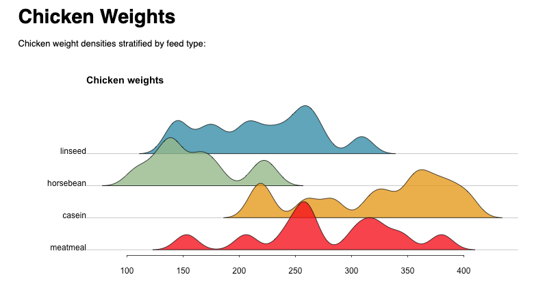
10. # Chicken Weights #
11.
12. Chicken weight densities stratified by feed type:
13.
14. ```{r plot, include=TRUE, echo=FALSE, fig.width=10, fig.height=5}
15. xs <- Map(getElement, dens, "x")
16. ys <- Map(getElement, dens, "y")
17. ys <- Map(function(x) (x-min(x)) / max(x-min(x)) * 1.5, ys)
18. ys <- Map(`+`, ys, length(ys):1)
19.
20. plot.new()
21. plot.window(xlim = range(xs), ylim = c(1,length(ys)+1.5))
22. abline(h = length(ys):1, col = "grey")
23.
24. invisible(
25. Map(polygon, xs, ys, col = hcl.colors(length(ys), "Zissou", alpha = 0.8))
26. )
27.
28. axis(1, tck = -0.01)
29. mtext(names(dens), 2, at = length(ys):1, las = 2, padj = 0)
30. title("Chicken weights", adj = 0, cex = 0.8)
31. ```
The first chunk calls redo-ifchange on all densities for selected feed types and reads their data into a list.
The second chunk produces a stacked density plot.
We can “knit” this file to produce the final html report.
Here I will be using the executable script that ships with the knitr(6) library but you can also produce the same report by calling knit() or render() from within R:
$ $R_LIBS_USER/knitr/bin/knit report.Rmd -o report.html

redo  soybean.density.rds
redo  meatmeal.density.rds
redo    meatmeal.subdata.rds
Again, from within the R-markdown script, redo was able to track the missing dependencies and compute them for us automatically. Here is a picture of the resulting document:
Now let’s make some changes.
Imagine we want to change the default bandwidth of our density estimating function.
In addition we also need to use horsebean instead of the soybean feed.
For this we have to change one line within default.density.rds.do file:
...
10.  dens <- density(rawdata$weight, bw=10)
...
And one line within 'report.Rmd':
...
2.   feeds <- c("linseed", "horsebean", "casein", "meatmeal")
...
And after compiling the report again only the needed dependencies will be re-executed:
$ $R_LIBS_USER/knitr/bin/knit report.Rmd -o report.html

redo  linseed.density.rds
redo  horsebean.density.rds
redo    horsebean.subdata.rds
redo  casein.density.rds
redo  meatmeal.density.rds
To better see the actions performed by the scripts and redo in the report execution completed above, here is a simplified call stack:
report.Rmd:                calls redo-ifchange linseed.density.rds
redo:                      finds the target linseed.density.rds
redo:                      checks linseed.density.rds dependencies
redo:                      detects a changed dependency: default.density.rds.do
redo:                      executes default.density.rds.do
default.density.rds.do:    calls redo-ifchange linseed.subdata.rds
redo:                      finds linseed.subdata.rds
redo:                      checks linseed.subdata.rds dependencies
redo:                      detects no changed dependencies
redo:                      halts
default.density.rds.do:    continues and produces the target linseed.density.rds
default.density.rds.do:    finishes
report.Rmd:                continues and calls redo-ifchange horsebean.density.rds
redo:                      cannot locate the target horsebean.density.rds
redo:                      looks for instruction file horsebean.density.rds.do
redo:                      cannot locate horsebean.density.rds.do
redo:                      looks for default instructions default.density.rds.do
redo:                      locates and executes default.density.rds.do
default.density.rds.do:    calls redo-ifchange horsebean.subdata.rds
redo:                      cannot locate the target horsebean.subdata.rds
redo:                      looks for instruction file horsebean.subdata.rds.do
redo:                      cannot locate horsebean.subdata.rds.do
redo:                      looks for default instructions default.subdata.rds.do
redo:                      locates and executes default.subdata.rds.do
default.subdata.rds.do:    calls redo-ifchange rawdata.rds
redo:                      finds rawdata.rds
redo:                      checks rawdata.rds dependencies
redo:                      detects no changed dependencies
redo:                      halts
default.subdata.rds.do:    continues and produces the target horsebean.subdata.rds
default.subdata.rds.do:    finishes.
default.density.rds.do:    continues and produces the target horsebean.density.rds
default.density.rds.do:    finishes
report.Rmd:                calls redo-ifchange casein.density.rds
...
The constructed analysis workflow is quite simple yet powerful.
If we were to make a change to this pipeline and run the redo command again it will make sure to only execute the parts that need to be redone.
In large projects this can save hours, days, or even weeks of computational time.
Importantly - we didn’t have to learn any new syntax or define special configuration files, the code we wrote was directly related to commands doing the work.
It also has to be said that redo is language agnostic and R, which was used here, can be replaced by any other language or even a mix of different languages.
Users can, for example, choose to do computation intensive tasks in C++, build a machine learning model with Python, and generate a report with R-markdown, all while working within the same framework of “redo”.
Finally a sobering thought - I only managed to touch on the basics of this elegant piece of software.
Those wanting to learn more are referred to documentation pages(7).